Many users cannot work with NetCDF data directly and need to extract data for a small region (perhaps a single grid cell) in plain text (ASCII) format. This document will walk you through extracting data from a NetCDF file into ascii format so that you can import it into Excel, or feed it into a modeling program, or even just look at the raw numbers.

Note: These instructions are for Windows users. If you are working on a linux, unix, or mac system, or if you have Cygwin installed, you have many more options. Probably the best is to install NCO and use the ncks command. For example: ncks -s "%f\n" -C -h -d xc,2,2 -d yc,3,3 -v tas datafile.nc
prints all the values for the variable tas at coordinates xc=2, yc=3 from datafile.nc, one per line (plus some metadata you can grep away if you don't want it). You can find a long list of useful tools on Unidata's NetCDF Software page.

Step-by-step instructions for converting NetCDF data to plain text

Step 1: Install the necessary tools

You will need to install two packages, NetCDF and FAN, to extract NARCCAP data to plain text on a Windows machine. In both cases, all you need to do is download the zip file, extract the files within, and place them in C:\Windows\System32. (You may need administrative privileges.)

Unidata's NetCDF package includes ncdump, which you can use to display the metadata from a NetCDF file. This is often very helpful for understanding how the data is organized inside the file. ncdump -h filename will display only the header information, without any of the actual data.

You can download the pre-built Win32 binary version of the netcdf library, including ncdump.exe, here: netcdf-3.6.1-beta1-win32dll.zip.

If you need more information about NetCDF on Windows, it can be found in Unidata's NetCDF Installation and Porting Guide.

The user-contributed FAN library, for extracting and manipulating array data from netCDF files, is also available from Unidata, on the User-Contributed netCDF Software page. To use FAN on a Windows machine, you'll want to download a pre-built binary: fan-2.0.3.win32bin.zip.

FAN includes nc2text.exe, which converts netCDF data to plain text. Extensive documentation can be found in Unidata's Introduction to FAN Language and Utilities.

Step 2: Figure out which grid cells you need

Data is stored in the NetCDF files in 2D arrays. To pull out data for a subregion, you need to know the appropriate range of array indices.

One important thing to note is that all the models use projected coordinate systems. The array dimensions are named "xc" and "yc" within the file. The grids are not square in lat/lon coordinates. Therefore, there are also 2D arrays named "lat" and "lon" that give the latitude and longitude for each grid cell.

If this is confusing, it may help to look at this grid point map, which shows the locations of all the grid cells for each of the RCMs. (It's a very high-resolution PDF, so you'll have to zoom in to make out individual points.)

To find the gridcells you need, just look up the indices on the following maps. Each PDF file is a map showing the locations of the grid cell centers for one of the models. Each grid cell has its array indices printed next to it. These are ridiculously high-resolution PDFs, so you'll have to zoom in to 1600% or higher to be able to discern the indices. The maps show state boundaries and major bodies of water and have graticule lines every 1 degree, so it should be relatively easy to find your region of interest.

Grid Cell Maps:
CRCM_points.pdf
ECP2_points.pdf
HRM3_points.pdf
MM5I_points.pdf
RCM3_points.pdf
WRFG_points.pdf

NOTE: Even if two models have grid cells in the same location, they won't necessarily have the same array indices! The models have different domain sizes due to differences in the sponge zone, and since the array indices are counted from the lower left corner, two models using the same map projection can still have different array numbering. Also be sure to sanity-check your numbers by looking at nearby grid cells. Because the map is at such high resolution, sometimes the numerals are a little hard to read. Double-check whether that's a 1 or a 4 you're looking at.

Data in the file is stored in the order [time,yc,xc]. Indices are given in the same order, so 15,20 on the map is yc=15, xc=20.

Step 3: Extract data from specified cells

Now that you have your array indices, you can extract data from the NetCDF file.

First, you need to get a command prompt. If you have a new Vista-style start menu, just enter cmd.exe in the search box; if you have a classic-style start menu, click "Run..." and enter cmd.exe in the dialog. This will open up the command-line interface, also known as the "DOS prompt".

Now, change directories in the command-line interface to wherever your NetCDF data is located. (For example, if you're running Vista and your data is on the desktop, you'd type cd C:\Users\username\Desktop .)

It will probably be helpful to have a look at how the data is organized. Type
ncdump -h filename
and you should get a page of output that looks something like this. This is the metadata for your file, telling you everything about how the data in the file is structured, like the names of the different variables, plus a lot of ancillary information such as units.

To extract the data, you just need to know the name of the variable and the array indices of the grid cell you want to extract. Give nc2text the filename, the variable, and the indices as shown in this example, redirecting the output to a text file using the > character:

nc2text pr_WRFG.nc pr[,yc=3,xc=5] > data.y3.x5.txt

This extracts all the values for variable 'pr' at coordinates 3,5 in the file 'pr_WRFG.nc' and prints them in plain text, one value per line, to the file 'data.y3.x5.txt'.

You can extract values for a range of coordinates, but if your range was, say, 2 cells high and 3 wide, the resulting output would be blocks of 2x3 numbers, separated by blank lines. You may find this format useful to view, but it's not very good for importing into programs like Excel, and you will in many cases be better off working with a separate file for each gridcell.

EXAMPLE

Let's say you're interested in climate in the eastern half of Nebraska. I'm going to run through an example for the point nearest the tri-state intersection of Nebraska, South Dakota, and Iowa—right near Sioux City.

Suppose we want to plot temperature versus time using Excel. It's always a good idea to sanity-check the data to make sure that the extracted values make numerical sense by doing something like making a simple plot.

First, install the NetCDF and FAN packages as described in step 1.

Then, download the data file. For this example, I'll use a small sample file containing only 50 timesteps: tas_WRFG_example.nc

Next, we find the indices of the grid cell of interest. Zooming in to 2400% magnification on the map, we find that the nearest gridpoint is slightly south and a little bit west of the point where the three state lines intersect. It has coordinates 43,67. Recall that these coordinates will only work for WRFG data; other models will have different gridcell coordinates for this location.

Now we open a command window and have a look at the headers. Navigate to the appropriate directory and run ncdump -h tas_WRFG_example.nc and you should see something that looks like this. We can see that the main data variable is named 'tas' and has units of degrees Kelvin.

We can now extract data for our location of interest and save it to a file:

nc2text tas_WRFG_example.nc tas[,yc=43,xc=67] > temp.csv

The first four values are: 253.657, 252.359, 250.731, and 249.935. The full output is here: temp.csv.

The resulting file can be opened in a spreadsheet program like Excel. Excel recognizes the .csv extension as a plain-text tabular data format where each line is a new row and columns are separated by commas. (The default output from nc2text puts a blank line between each number; if that's inconvenient, you can Google "excel remove blank lines" to find lots of macros that will fix it, or just open up the file in something like Word and get rid of the blank lines with a search-and-replace.)

Then we'll do something similar for time:

nc2text -n 1 -f %.3f tas_WRFG_example.nc time[] > time.csv

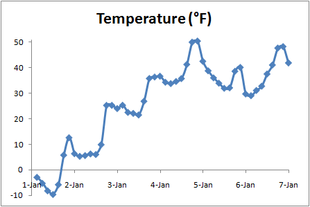
Here's the full result: time.csv.

The "-n 1" flag in the command tells nc2text to put only one value per line. (We need it for time because it's a one-dimensional variable.) "-f %.3f" ensures that there are three places after the decimal (otherwise we'd get rounding errors, because the data are 8x-daily). Time in the NARCCAP data is stored as hours elapsed since a baseline, specified in the metadata. In our example, it is 1979/01/01 00:00 UTC. So when you open this file in Excel, you can convert from hours to dates by entering the baseline date into a cell and adding the time values as offsets to it.

Converting temperature from Kelvin to the more familiar degrees Fahrenheit and plotting against time, we can see the clear daily signal of daytime highs and nighttime lows in a range that is reasonable for early January in this part of the world: